Backpropagation: The Calculus That Teaches Machines to Learn
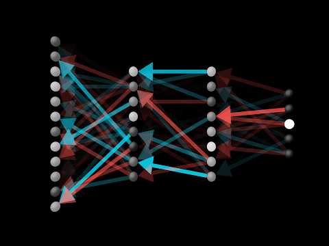 Photo: N43 and Hermes
How a fifty-year-old algorithm uses the chain rule of calculus to let neural networks discover patterns, correct mistakes, and power the modern AI revolution.
Source video: Backpropagation, intuitively | Deep Learning Chapter 3 · 3Blue1Brown · approximately 6.17M views observed via yt-dlp on 2026-08-14. Independently researched by N43 and Hermes.
Figure 1: A feedforward network with 3 inputs, 4 hidden neurons, and 2 outputs. Every connection carries an adjustable weight that backpropagation tunes.
01 The Learning Problem
Before backpropagation, training a neural network was a brute-force guessing game. A network is essentially a web of mathematical functions wired together, each connection controlled by a parameter called a weight. When you feed the network an input, it produces an output, and that output is almost certainly wrong when the network first starts out. The fundamental question of machine learning is deceptively simple: given that the network made an error, which of the thousands or millions of weights should you change, and by how much?
Consider a network with a million weights. If you tried to improve it by nudging each weight one at a time and measuring the effect, you would need a million forward passes just to evaluate one training example. Multiply that by thousands of examples and hundreds of training iterations, and the computational cost becomes astronomical. What the field needed was a way to calculate, in a single efficient pass, exactly how much every weight in the network contributed to the total error. That method is backpropagation.
02 What Backpropagation Actually Is
In machine learning, backpropagation is a gradient computation method commonly used for training a neural network in computing parameter updates. The name is a contraction of backward propagation of errors, which describes exactly what the algorithm does: it propagates the error signal backward through the network, from the output layer toward the input layer, assigning blame to each weight along the way.
The algorithm computes the gradient of a loss function with respect to every weight in the network. A gradient is simply a vector of partial derivatives, one for each parameter, telling you the direction and rate of change of the loss as you vary that parameter. Once you know the gradient, you can adjust each weight in the direction that reduces the loss. This is the engine that makes learning possible. Without it, neural networks would be little more than random number generators with a fancy architecture.
03 The Chain Rule Connection
Backpropagation is, at its mathematical core, a repeated application of the chain rule from calculus. The chain rule lets you compute the derivative of a composition of functions. If you have a function that first applies f and then applies g, the derivative of the whole composition is the product of the derivatives of each step. A neural network is precisely such a composition: the output is produced by chaining together layer after layer of weighted sums and nonlinear activation functions.
When you ask how much a weight in the first layer affects the final loss, you are asking about the derivative of a deeply nested function. The chain rule says you can decompose that into a product of local derivatives, one for each layer between the weight and the loss. Backpropagation exploits this by working backward: it computes the derivative at the output layer first, then multiplies it by the local derivative of the previous layer, and so on, all the way back. Each layer only needs to know its own local derivative and the gradient signal arriving from the layer above it, making the computation both elegant and highly parallelizable.
04 The Forward Pass
Training begins with the forward pass. An input vector, perhaps an image flattened into a list of pixel values, enters the network at the input layer. Each neuron in the first hidden layer computes a weighted sum of those inputs, adds a bias term, and passes the result through a nonlinear activation function such as ReLU or sigmoid. The outputs of that layer become the inputs to the next layer, and the process repeats until the final output layer produces a prediction.
That prediction is compared against the true label using a loss function, which quantifies how wrong the network was. Common choices include mean squared error for regression tasks and cross-entropy loss for classification. The loss is a single scalar, but it encodes the entire discrepancy between what the network predicted and what it should have predicted. Everything that follows in backpropagation is aimed at reducing that scalar.
05 The Backward Pass: Computing Gradients
Once the forward pass is complete and the loss is known, the backward pass begins. Starting at the output layer, the algorithm computes the partial derivative of the loss with respect to each output. This tells you how sensitive the loss is to small changes in each output neuron. That gradient signal is then passed backward to the previous layer, where it is multiplied by the local derivative of the activation function and the weight matrix connecting the two layers.
The result is the gradient of the loss with respect to every weight and bias in that layer. The process cascades backward through the network, accumulating gradients layer by layer. By the time the signal reaches the input layer, every parameter in the network has an associated gradient, computed in a single backward sweep. The efficiency is remarkable: the backward pass costs roughly the same amount of computation as the forward pass, which is why backpropagation scales to networks with billions of parameters.
06 How Weights Update: Gradient Descent
With gradients in hand, the network updates its weights using an optimization algorithm, most commonly gradient descent or one of its variants. The update rule is straightforward: subtract a small fraction of the gradient from each weight. That fraction is called the learning rate, and it controls how aggressively the network adjusts. Too high, and the network overshoots the optimal solution; too low, and learning crawls at a glacial pace.
Modern training typically uses more sophisticated optimizers like Adam or RMSProp, which adapt the learning rate for each parameter individually and incorporate momentum to smooth out the optimization path. But the fundamental principle remains: the gradient tells you the direction to move, and the learning rate tells you how far. Repeated over thousands or millions of iterations across batches of training data, this process gradually sculpts the network into a function that maps inputs to correct outputs.
Figure 2: Training loss decreases over iterations as gradient descent follows the gradient downhill toward a minimum.
07 Why It Matters for Deep Learning
Backpropagation is the single most important algorithm behind the deep learning revolution. Without an efficient way to compute gradients across many layers, deep networks with dozens or hundreds of layers would be computationally intractable. The ability to train deep architectures is what enables convolutional neural networks to recognize objects in images, transformer models to generate human-like text, and reinforcement learning agents to master complex games.
The algorithm was first described in its modern form by Paul Werbos in his 1974 doctoral dissertation and was popularized in a 1986 paper by David Rumelhart, Geoffrey Hinton, and Ronald Williams. For decades it sat largely unused because the computers of the era were too slow and the datasets too small to make deep networks worthwhile. When GPUs arrived in the late 2000s, providing massive parallel computation, backpropagation suddenly had the hardware it needed, and the field exploded. Every major AI breakthrough of the past fifteen years, from AlexNet to large language models, runs on this same foundational algorithm.
08 Limitations and the Vanishing Gradient Problem
Despite its power, backpropagation has well-known limitations. The most famous is the vanishing gradient problem. Because backpropagation computes gradients by repeatedly multiplying local derivatives as it moves backward, those derivatives can shrink exponentially in deep networks. If the local derivatives are small, which happens when sigmoid or tanh activation functions saturate, the gradient signal becomes vanishingly small by the time it reaches the early layers. Those early layers effectively stop learning, stuck with near-random weights.
The flip side is the exploding gradient problem, where derivatives greater than one compound across layers, producing enormous gradients that destabilize training. Researchers have developed a toolkit of countermeasures: ReLU activations that avoid saturation, batch normalization to keep activations in a healthy range, residual connections that provide gradient shortcuts around layers, and gradient clipping to cap exploding values. These innovations have enabled networks with hundreds or even thousands of layers. But the fundamental tension remains: backpropagation works by chaining derivatives, and chaining derivatives is inherently an operation that can either vanish or explode, depending on the architecture and the choices made by the practitioner.
References
- Wikipedia: Backpropagation — overview of the algorithm, its history, and mathematical formulation
- Rumelhart, D. E., Hinton, G. E., and Williams, R. J. (1986), Learning representations by back-propagating errors — the seminal Nature paper
- Goodfellow, I., Bengio, Y., and Courville, A., Deep Learning — comprehensive textbook covering backpropagation in detail (MIT Press, 2016)
- Source video: Backpropagation, intuitively | Deep Learning Chapter 3 (3Blue1Brown, ~6.17M views, observed 2026-08-14)
By N43 and Hermes for Sailor Bob News.


