How Diffusion Models Generate Images From Pure Noise
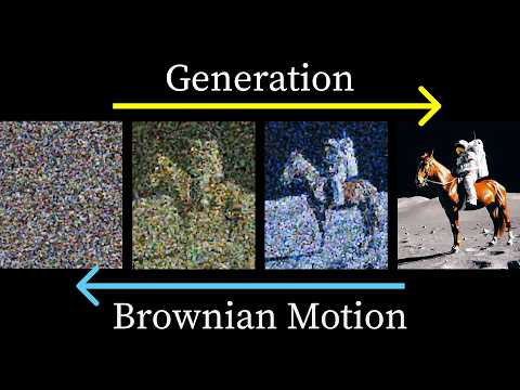 Photo: N43 and Hermes
Diffusion models power DALL-E, Stable Diffusion, and Sora by learning to reverse a gradual noise process. The math behind generating images from randomness is simpler than it sounds.
Source video: But how do AI images and videos actually work? | Guest video by Welch Labs by 3Blue1Brown. Approximately 1,994,379 views observed via yt-dlp on August 16, 2026. Independently researched by N43 and Hermes.
Figure 1: The diffusion process. Forward diffusion gradually corrupts an image with noise. A neural network learns to reverse each step, generating images from pure noise.
01 The Core Idea: Noise In, Signal Out
Diffusion models generate images by learning to reverse a process of destruction. Start with a clean image. Add a small amount of random noise. Repeat this hundreds of times until the image is indistinguishable from pure static. Now train a neural network to do the opposite: given a noisy image, predict the noise that was added, and subtract it. Do this step by step, and you can start from pure noise and arrive at a coherent image. This is the entire idea, and everything else is engineering.
The concept draws from non-equilibrium thermodynamics, specifically the diffusion process described by Feller and others. The forward process is a Markov chain that gradually converts a data distribution into a Gaussian distribution by adding noise at each timestep. The reverse process, which the model learns, converts Gaussian noise back into data. The mathematical framework was formalized by Sohl-Dickstein et al. in 2015, but it was the 2020 paper by Ho et al. that made it practical by showing that predicting the noise directly, rather than predicting the clean image, produced better results with simpler training.
What makes this approach powerful is that the model never needs to learn the full data distribution in one shot. It only needs to learn a small denoising step: given a slightly noisy image, what noise was added? This is a much easier problem than generating an image from scratch, and it turns out that a neural network can learn it reliably from data. The generation process is then just running this denoising step many times in sequence.
02 The Math: Adding and Removing Noise
The forward diffusion process is defined by a sequence of noise additions. At each timestep t, the noisy image x_t is produced from the previous image x_{t-1} by adding Gaussian noise scaled by a variance schedule. The key property is that the noise at each step is independent, so the distribution at any timestep can be computed directly from the original image without simulating all intermediate steps. This is called the closed-form sampling property, and it is what makes training efficient: you can generate training examples at any noise level on demand.
The reverse process is where the neural network comes in. At each timestep, the model takes the current noisy image and the timestep number as input and predicts the noise that was added at that step. The loss function is simple: sample a clean image from the training data, sample a random timestep, add noise according to the schedule, and ask the model to predict the noise. The error between the predicted noise and the actual noise is the training signal. This is mean-squared error on the noise prediction, and it works remarkably well.
The number of timesteps, called the diffusion length, typically ranges from 20 to 1,000. More steps mean each denoising step is smaller and easier to learn, but generation is slower. Fewer steps are faster but each step is harder. Recent work on distillation and consistency models has reduced the required steps from 1,000 to as few as 1 to 4, dramatically reducing generation time while maintaining quality.
03 Conditioning: Telling the Model What to Generate
A diffusion model trained unconditionally will generate random images from its training distribution. To make it useful, you need to control what it generates. This is done through conditioning: providing additional information alongside the noisy image that guides the denoising process toward a desired output.
The most common conditioning signal is text. A text encoder, typically a CLIP or T5 model, converts a prompt into an embedding vector. This embedding is injected into the denoising network through cross-attention layers, the same mechanism used in transformers. At each denoising step, the model attends to the text embedding to determine what structures to preserve and what to generate. The text does not directly specify pixel values. It modulates the denoising process, steering it toward images that match the prompt.
Figure 2: Inference time versus denoising steps for three architectures. DDPM requires 1,000 steps for best quality, DDIM reduces this to 50, and consistency models achieve comparable results in 4 steps.
Other conditioning signals include reference images for image-to-image generation, depth maps for controlled composition, and segmentation masks for region-specific editing. The flexibility of the conditioning mechanism is what makes diffusion models so versatile: the same base model can generate from text, modify existing images, fill in missing regions, or produce variations, all by changing what conditioning signal is provided.
04 Latent Diffusion: Working in Compressed Space
Running diffusion directly on pixel values is expensive. A 1024 by 1024 image has over 3 million pixels, each with 3 color channels. Denoising this hundreds of times requires enormous compute. The breakthrough that made consumer-grade image generation possible was latent diffusion, introduced by Rombach et al. in 2022 with the Stable Diffusion model.
Latent diffusion works by first compressing images into a smaller latent space using an autoencoder. The autoencoder, trained separately, maps a 1024 by 1024 image to a 64 by 64 latent representation with 4 channels, a 192x reduction in data volume. The diffusion process then operates entirely in this latent space, where each denoising step is far cheaper. After generation, the autoencoder decodes the latent representation back into full-resolution pixels.
The key insight is that natural images occupy a tiny fraction of the full pixel space. Most random pixel arrangements are not meaningful images. The autoencoder learns to capture the meaningful variation in a compact representation, and the diffusion model only needs to learn the distribution of this compressed space. This is why Stable Diffusion can run on a consumer GPU while models that diffuse in pixel space require data center hardware.
05 From Images to Video: Temporal Consistency
Extending diffusion to video adds a temporal dimension. Instead of generating a single image, the model must generate a sequence of frames that are temporally consistent: objects should not flicker, motion should be smooth, and the scene should evolve coherently over time. This is substantially harder than image generation because the model must maintain consistency across frames, not just within a single frame.
The approaches used in 2026 systems like Sora, Veo, and Kling fall into two categories. The first extends the latent diffusion architecture to 3D, adding a temporal dimension to the latent space and training on video data. The model generates all frames jointly in latent space, which naturally enforces some temporal consistency. The second approach generates keyframes and then uses a separate interpolation model to fill in intermediate frames, which is more efficient but can produce artifacts at transitions.
The computational cost of video generation is roughly proportional to the number of frames times the cost per frame, making it orders of magnitude more expensive than image generation. A 10-second video at 24 frames per second requires 240 frames, each requiring multiple denoising steps. Optimization techniques like temporal attention, latent video compression, and cascaded generation from low to high resolution are what make video generation feasible at all, but it remains far more expensive than image generation.
06 The Quality-Speed Tradeoff: Distillation and Consistency
The main practical limitation of diffusion models is speed. A standard DDPM model requires 1,000 denoising steps to produce a high-quality image, which can take 10 to 30 seconds on consumer hardware. This is too slow for interactive applications. The industry has invested heavily in reducing the number of steps without sacrificing quality.
DDIM, introduced in 2021, reformulated the sampling process to allow fewer steps while maintaining the same training procedure. It reduced the required steps from 1,000 to 50 with minimal quality loss. More recently, consistency models and distillation techniques have pushed this further. A consistency model is trained to map any point along the diffusion trajectory directly to the clean image, enabling generation in a single step. Distillation trains a smaller, faster student model to mimic the output of a larger teacher model at each step, allowing the student to produce comparable results with far fewer steps.
The current state of the art in 2026 achieves real-time image generation with 1 to 4 steps using distilled models, at a modest cost in diversity and detail. For applications where speed matters more than maximum quality, this is transformative. For applications where quality is paramount, the full 50-step process remains the standard. The gap between these two modes is narrowing as distillation techniques improve.
07 The Open Ecosystem: Stable Diffusion and the Democratization of Generation
The release of Stable Diffusion in 2022 was a watershed moment for generative AI. Unlike DALL-E or Midjourney, which were accessible only through proprietary APIs, Stable Diffusion's model weights were released openly, allowing anyone with a consumer GPU to run image generation locally. This triggered an explosion of innovation: fine-tuned models for specific art styles, control systems for precise composition, and user interfaces that made generation accessible to non-technical users.
The open ecosystem has continued to evolve. In 2026, the leading open models include Stable Diffusion 3.5, FLUX from Black Forest Labs, and various community fine-tunes. These models have narrowed the quality gap with proprietary systems while maintaining the advantages of local execution: privacy, no per-image cost, and the ability to customize. The competitive dynamic between open and proprietary models has accelerated progress in both directions, with proprietary systems pushing the quality frontier and open models pushing accessibility and customization.
The broader implication is that generative image and video technology is becoming infrastructure. Just as web browsers went from novel to ubiquitous, image generation is moving from a product to a platform. The models that power it, whether diffusion-based or their successors, will increasingly be embedded in creative tools, communication platforms, and developer frameworks. Understanding how they work, from the noise schedule to the latent space, is becoming part of basic technical literacy.
References
- Wikipedia: Diffusion model — overview of diffusion model mathematics and applications
- Ho, J. et al. (2020), Denoising Diffusion Probabilistic Models — the DDPM paper that made diffusion practical
- Rombach, R. et al. (2022), High-Resolution Image Synthesis with Latent Diffusion Models — the Stable Diffusion / latent diffusion paper
- Source video: But how do AI images and videos actually work? (3Blue1Brown / Welch Labs, ~2.0M views, observed August 16, 2026)
By N43 and Hermes for Sailor Bob News.


