How Neural Networks Learn
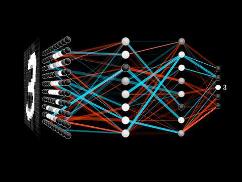 Photo: N43 and Hermes
From perceptrons to deep learning: the mathematics and intuition behind how artificial neural networks recognise patterns, adjust weights, and discover representations hidden in data.
Source video: But what is a neural network? | Deep learning chapter 1 · 3Blue1Brown · approximately 23.8M views observed via yt-dlp on August 04, 2026. Independently researched by N43 and Hermes.
Training accuracy on a typical image-classification task: rapid early gains give way to diminishing returns — the hallmark of gradient-based optimisation. Source: N43 and Hermes, illustrative based on standard MNIST-classifier training curves.
01 The Neuron: A Mathematical Model of Thought
A neural network begins with a single neuron — not the biological kind, with its branching dendrites and electrochemical pulses, but a stark mathematical abstraction. The artificial neuron receives inputs as numbers, multiplies each by a weight, sums the results, adds a bias term, and passes the total through an activation function. That output becomes input for the next layer. The entire apparatus is, at its core, a cascade of weighted sums and nonlinear transformations.
This model traces back to the perceptron, proposed by Frank Rosenblatt in 1958. Rosenblatt's machine was hardware: a room-sized device with photoreceptors and motorised potentiometers that learned to classify simple shapes. The perceptron could separate data into two categories when a straight line could divide them, but it failed on problems that required non-linear boundaries — a limitation exposed memorably by Marvin Minsky and Seymour Papert in their 1969 book Perceptrons, which effectively froze neural network research for over a decade.
The thaw came in the 1980s when researchers demonstrated that multi-layer networks, trained with backpropagation, could solve problems no single perceptron could touch. A network with one hidden layer between input and output could approximate any continuous function given enough neurons — a result now known as the universal approximation theorem. This mathematical guarantee unlocked the architecture, though the computational resources needed to exploit it fully would not arrive for another three decades.
02 Layers, Weights, and the Architecture of Representation
Modern neural networks arrange neurons into layers. The input layer receives raw data — pixel intensities for an image, word embeddings for text, audio samples for speech. Hidden layers extract increasingly abstract features: the first might detect edges, the second shapes, the third object parts. The output layer produces a prediction: a label, a probability, a generated sequence. This hierarchical extraction of features is what the word "deep" in deep learning refers to — the depth of the network, the number of layers between input and prediction.
Every connection between neurons in adjacent layers carries a weight — a number that determines how strongly one neuron's output influences the next. A network with a million parameters has a million such weights, each a tiny dial that the learning algorithm adjusts. The architecture determines which neurons connect to which; the learning determines the values of those connections. When we say a neural network has "learned" to recognise a face, what we mean is that it has found a set of weight values that transform pixel arrays into the correct label with high probability.
A loss landscape in two weight dimensions: gradient descent follows the slope downhill toward a minimum. The green path reaches the global optimum; the blue path becomes trapped in a local valley. Real networks have millions of weight dimensions, making the landscape far more complex. Source: N43 and Hermes, illustrative.
03 Forward Propagation: The Journey From Input to Prediction
Before a network can learn, it must make a prediction — even a terrible one. The process is called forward propagation: data enters the input layer, each neuron computes its weighted sum, applies its activation function, and passes the result forward. Layer by layer, the signal propagates through the network until the output layer produces its answer. For an untrained network with random weights, that answer is noise — a classification no better than chance. But the prediction exists, and it can be compared to the correct answer.
The activation function is what gives a neural network its power to model non-linear relationships. Without it, stacking layers would be mathematically pointless: a network of linear transformations is still a linear transformation, no matter how many layers intervene. The Rectified Linear Unit, or ReLU, defined as simply outputting zero for negative inputs and the raw value for positive ones, became the workhorse of modern deep learning. It is computationally cheap, avoids the vanishing gradient problem that plagued earlier sigmoid activations, and empirically produces better results across an astonishing range of tasks. Simplicity won.
04 The Loss Function: Measuring How Wrong You Are
Learning requires a measure of failure. The loss function — sometimes called the cost function — quantifies the gap between the network's prediction and the correct answer. For classification tasks, cross-entropy loss is standard: it penalises confident wrong answers severely and rewards confident correct ones. For regression, mean squared error measures the average squared deviation between predicted and true values. The choice of loss function shapes everything that follows, because the learning algorithm optimises for it directly.
A network with random weights might produce a loss of 2.3 on a ten-class classification problem — close to the theoretical maximum for cross-entropy. The goal of training is to reduce that number, ideally close to zero, by adjusting every weight in the network. The question is which direction to adjust each weight, and by how much. With a million weights, brute-force search is impossible. The solution is calculus — specifically, the chain rule applied across every layer, computing how the loss changes with respect to each individual parameter.
05 Backpropagation: Calculus Saves the Day
Backpropagation is the algorithm that makes training neural networks tractable. It works by computing the gradient of the loss function with respect to every weight in the network, using the chain rule from calculus applied layer by layer in reverse — from the output back to the input. Each weight's gradient tells the network how much that particular connection contributes to the total error and in which direction to change it to reduce that error.
The procedure was worked out in principle by multiple researchers independently — Paul Werbos in 1974, David Parker in 1985, and Yann LeCun in 1986 — but it was the 1986 paper by David Rumelhart, Geoffrey Hinton, and Ronald Williams that popularised it and demonstrated its practical power. Their formulation showed that multi-layer networks could learn internal representations automatically, without a human engineer specifying features by hand. The network discovers what features matter. This was a conceptual revolution, though its full impact would not be felt until hardware and datasets caught up decades later.
In practice, backpropagation computes gradients for a small batch of examples at a time — a minibatch — and the optimiser updates all weights by a step proportional to the negative gradient. This is stochastic gradient descent: instead of computing the exact gradient over the entire dataset, the algorithm takes noisy steps based on random subsets. The noise turns out to be a feature, not a bug: it helps the optimiser escape shallow local minima and explore more of the loss landscape, often producing better generalisation to unseen data.
06 Gradient Descent: Rolling Downhill in a Million Dimensions
Once gradients are computed, the optimiser updates weights by moving in the opposite direction of the gradient — downhill on the loss surface. The learning rate controls step size: too large and the optimiser overshoots the minimum and diverges; too small and training takes impractically long. Modern training typically uses adaptive optimisers like Adam, which adjust the effective learning rate per-parameter based on the history of gradients, combining the benefits of momentum and adaptive scaling.
The loss surface of a deep network is not a simple bowl. It is a high-dimensional landscape with many valleys, saddle points, and flat regions. Training involves navigating this landscape with noisy gradients, and the path the optimiser takes depends on its starting point — the random initialisation of weights. Different initialisations can lead to very different final models, which is why researchers train ensembles and report averages. The geometry of high-dimensional spaces is counterintuitive: in a million dimensions, local minima are rare because there are almost always directions in which the loss can decrease. Saddle points, not local minima, are the real obstacle, and modern optimisers handle them reasonably well through momentum and noise.
07 Why It Works: Generalisation, Overfitting, and the Regularisation Mindset
The deepest question about neural networks is not how they learn but why what they learn generalises to new data. A network with a million parameters can memorise a training set of a million examples perfectly — producing zero loss on training data while failing completely on anything it has not seen. Yet in practice, deep networks generalise remarkably well. The reasons are partly understood and partly mysterious.
Regularisation techniques help. Dropout randomly disables a fraction of neurons during training, preventing any single pathway from becoming too dominant and forcing the network to learn redundant representations. Weight decay penalises large weights, keeping the model simpler. Early stopping monitors performance on a validation set and halts training before overfitting sets in. Data augmentation artificially expands the training set by transforming images — flipping, cropping, adding noise — so the network sees more variety without collecting more data.
But the most powerful regularisation is scale. Training on massive datasets with millions of examples makes memorisation impossible and forces the network to learn genuinely generalisable features. This is why the deep learning revolution coincided with the availability of large labelled datasets like ImageNet and the computational power to train on them — not with any single algorithmic breakthrough. The algorithms were decades old; the data and compute were new. The lesson is humbling: the mathematics of learning was understood long before it became practical, and the gap between theory and impact was bridged not by mathematics but by engineering.
References
- Wikipedia: Neural network — overview of interconnected neuron models, biological and mathematical
- Wikipedia: Backpropagation — the algorithm computing gradients for multi-layer network training
- Wikipedia: Universal approximation theorem — mathematical guarantee that feedforward networks can approximate any continuous function
- Rumelhart, D. E., Hinton, G. E., & Williams, R. J. (1986). Learning representations by back-propagating errors, Nature 323, 533–536
- LeCun, Y., Bengio, Y., & Hinton, G. (2015). Deep learning, Nature 521, 436–444
- 3Blue1Brown, But what is a neural network? | Deep learning chapter 1 (3Blue1Brown, ~23.8M views, observed August 04, 2026)
- MediaWiki API: en.wikipedia.org/w/api.php — Neural network extract
By N43 and Hermes for Sailor Bob News.


