How Neural Networks Learn: The Mathematics Behind Machine Intelligence
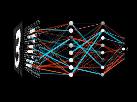 Photo: N43 and Hermes
From simple neurons to deep learning networks, the mathematical principles that enable machines to recognize patterns, process language, and make predictions.
Source video: But what is a neural network? | Deep learning chapter 1 · 3Blue1Brown · approximately 23.8M views observed via yt-dlp on 2026-08-11. Independently researched by N43 and Hermes.
01 What a Neuron Actually Computes
An artificial neuron is not a metaphor. It is a mathematical function that takes several numbers as input, multiplies each by a corresponding weight, adds a bias term, and passes the result through a nonlinear activation function. The output is a single number. The name comes from a loose analogy with biological neurons, which fire when the sum of their inputs crosses a threshold, but the mathematical object does not need biology to justify it.
What makes this simple operation powerful is that the weights are adjustable. When a neural network learns, it is adjusting the values of these weights, nudging each one slightly so that the network's overall output moves closer to a desired result. A single neuron can solve trivial problems like classifying whether a point is above or below a line. But when millions of neurons are arranged in layers and connected to one another, the combined function they compute becomes expressive enough to recognize faces, translate languages, and predict the next word in a sentence.
The key insight is that learning is optimization. The network does not discover rules in a human-like way. It descends a high-dimensional landscape of possible weight configurations, searching for the valley where errors are smallest. Every parameter the network contains is one dimension of that landscape, and modern networks have billions of them.
02 The Architecture of Layers
Neural networks are organized into layers. The first layer receives the raw input data, the last layer produces the output, and the layers between them are called hidden layers. Each neuron in a hidden layer receives signals from every neuron in the previous layer, computes its weighted sum, applies its activation function, and passes the result forward. This is what the term fully connected means, and it was the dominant architecture until the early 2010s.
The depth of a network, the number of hidden layers it contains, turned out to matter enormously. Shallow networks with one or two hidden layers can approximate any continuous function given enough neurons, a result formalized in the universal approximation theorem. But shallow networks need exponentially more neurons to achieve what a deep network can do with far fewer parameters. Depth allows the network to build hierarchical representations: early layers detect edges, middle layers detect shapes and textures, and later layers detect objects and concepts. This compositional structure mirrors how visual cortex processes information in biological brains, though the parallel is functional rather than anatomical.
03 How Weights and Biases Shape Output
Every connection between neurons has a weight, and every neuron has a bias. These two types of parameters are what the network learns. The weight controls how much influence one neuron's output has on another, while the bias shifts the activation function's threshold, determining how easily the neuron fires regardless of its inputs.
Consider a network trained to classify handwritten digits. Each pixel in the input image connects to every neuron in the first hidden layer, and each connection has its own weight. After training, some weights will be large and positive for pixels that strongly indicate a particular digit, others will be large and negative for pixels that argue against it, and many will be near zero for pixels that carry little signal. The bias for each neuron determines its baseline level of activation, allowing it to be selective or permissive depending on what features it has learned to detect.
The sheer number of parameters is what gives large networks their flexibility. A network with 175 billion parameters, like the GPT-3 language model, has a 175-billion-dimensional space of possible configurations. Training is the process of navigating that space to find a point where the network performs well on the task it was given.
04 Activation Functions and Nonlinearity
Without nonlinear activation functions, a neural network would be nothing more than a series of matrix multiplications. No matter how many layers you stack, the composition of linear functions is still linear, and a linear function can only model straight-line relationships. The activation function is what breaks that constraint and gives the network the ability to model curves, discontinuities, and complex decision boundaries.
The rectified linear unit, or ReLU, is the most widely used activation function in modern deep learning. It is defined as the maximum of zero and the input, meaning any negative value becomes zero and any positive value passes through unchanged. ReLU is simple, fast to compute, and its derivative is either zero or one, which makes gradient-based optimization efficient. Earlier activation functions like the sigmoid and hyperbolic tangent squashed their outputs into narrow ranges, which caused gradients to vanish as they propagated backward through many layers. ReLU largely solved this problem and made it practical to train networks with dozens or hundreds of layers.
05 Backpropagation and Gradient Descent
Training a neural network requires two things: a way to measure how wrong the network's predictions are, and a way to adjust the weights to make them less wrong. The first is the loss function, which computes a single number representing the error between the network's output and the correct answer. The second is backpropagation, the algorithm that calculates how much each weight contributed to the error and which direction to change it.
Backpropagation applies the chain rule from calculus repeatedly, starting from the output layer and working backward through the network. At each layer, it computes the gradient of the loss with respect to every weight and bias. These gradients tell the optimizer how to change each parameter to reduce the error. The optimizer then takes a small step in the direction the gradients point, a process called gradient descent. The size of that step is the learning rate, one of the most critical hyperparameters in training.
In practice, the process repeats millions of times across batches of training data. Each pass adjusts weights incrementally, and over many epochs the network's predictions improve. The gap between training accuracy and validation accuracy, visible in the chart above, reveals whether the network is overfitting to its training data or learning patterns that generalize to new examples. A network that memorizes training data perfectly but fails on validation has not learned anything useful, it has merely stored the answers.
06 Why Deep Networks Are Powerful
Deep networks outperform shallow ones not because they have more parameters in aggregate, but because depth creates compositional structure. Each layer transforms the representation it receives into something slightly more abstract, and each subsequent layer builds on that abstraction. A network trained to recognize objects in images learns edges in its first layer, corners and textures in the second, object parts in the third, and whole objects in deeper layers. This hierarchy means that features learned for one task can often be transferred to another, a technique called transfer learning that has become one of the most practical tools in modern machine learning.
The transformer architecture, introduced in 2017 for language translation, took this principle to an extreme. Transformers process sequences using a mechanism called self-attention, which allows every position in a sequence to attend to every other position, regardless of distance. This removed the sequential bottleneck of recurrent networks and made it possible to train models with hundreds of layers on massive text corpora. The results were large language models like GPT, Claude, and Gemini, which demonstrate that scaling up depth, width, and data produces qualitatively new capabilities.
07 The Limits and Future of Neural Network Architectures
Neural networks are powerful but not magical. They require large amounts of labeled data or carefully designed self-supervised objectives. They can be fooled by adversarial examples, inputs that are imperceptibly different from real data but cause the network to produce wildly wrong outputs. They inherit biases from their training data, and they lack the causal reasoning that would let them understand why things happen rather than merely correlating patterns.
The field is also confronting the energy cost of training and running large models. A single training run of a frontier language model can consume megawatt-hours of electricity and produce tons of carbon emissions. Researchers are exploring more efficient architectures, quantization techniques that reduce precision without sacrificing performance, and analog computing approaches that could perform matrix operations with far less energy. The mathematical foundations remain the same: neurons compute weighted sums, activation functions introduce nonlinearity, and backpropagation adjusts parameters. What is changing is the scale at which these principles are applied and the hardware that runs them.
References
- Wikipedia: Neural network — overview of biological and artificial neural networks, their mathematics and applications
- Wikipedia: Backpropagation — the algorithm for computing gradients in neural networks
- 3Blue1Brown, But what is a neural network? | Deep learning chapter 1 (~23.8M views, observed 2026-08-11)
- Stanford CS231n, Convolutional Neural Networks for Visual Recognition — university course notes on neural network architectures
By N43 and Hermes for Sailor Bob News.


