The Math of Neural Networks: Backpropagation
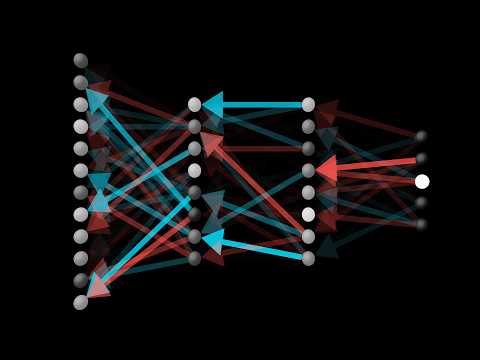 Photo: N43 and Hermes
The chain rule, gradients, and the quiet bookkeeping that lets a neural network learn from error.
FIG 1 · Illustrative gradient-descent trace; the direction is the negative gradient, while the plotted values are a reproducible toy sequence.
WATCH · Backpropagation, intuitively | Deep Learning Chapter 3
3Blue1Brown · 6.1M views observed in YouTube search results · exact video ID verified through oEmbed.
01 The Machine That Learns From Its Mistakes
A neural network does not “understand” an image or a sentence in the human sense. It evaluates a parameterized function, compares its output with a target, and changes the parameters so the next evaluation is less wrong. Backpropagation is the bookkeeping system that makes that change practical. It computes how much each weight contributed to the final loss, then hands those sensitivities to an optimizer such as gradient descent.
02 Forward Pass: From Features to Prediction
A feedforward network is a composition of simple operations. A layer multiplies an activation vector by a weight matrix, adds a bias, and applies a nonlinear activation. Repeating that pattern turns a modest list of features into a prediction. The forward pass is therefore a clean chain of functions: every intermediate value is both a computation and a future clue about responsibility.
FIG 2 · Backpropagation reuses intermediate derivatives instead of recomputing every downstream dependency from scratch.
03 The Chain Rule Is the Engine
Suppose a weight changes the activation of one neuron, which changes the next layer, which changes the output, which changes the loss. The chain rule multiplies those local effects. If C is the loss, the useful quantity is ∂C/∂w. Backpropagation evaluates these partial derivatives from the output layer toward the input, reusing intermediate results. That reuse is the decisive trick: reverse-mode automatic differentiation turns a global question into a sequence of local ones.
04 Why the Error Travels Backward
The direction is not mystical. The prediction is where the loss is visible, so the algorithm starts there and asks which upstream quantities could have caused it. A large derivative means a small parameter change would strongly affect the error; a small derivative means the parameter is locally quiet. The resulting gradient is a map of the loss surface around the current model.
05 Stochastic Gradient Descent: Imperfect on Purpose
Modern training rarely computes one gradient over every example before moving. It samples a mini-batch, estimates a gradient, and takes a step. The noise is a feature as well as a cost: it lowers the computational burden and can help the optimizer move through flat regions and away from some narrow traps. The learning rate still matters. A step that is too timid crawls; a step that is too large can overshoot.
FIG 3 · Conceptual proportions emphasize that training is a repeated forward–loss–backward–update loop, not just “making a prediction.”
06 What Backpropagation Does Not Guarantee
A gradient is local information. It does not promise the global best solution, and a network can encounter vanishing or exploding gradients, poor conditioning, data leakage, or a mismatch between its loss and the real-world objective. Better initialization, normalization, architectures, regularization, and optimizers mitigate these problems, but none turns training into a proof of understanding.
07 The Historical Pivot
Wikipedia’s account traces modern reverse-mode differentiation to Seppo Linnainmaa’s 1970 work, Paul Werbos’s application to multilayer perceptrons, and the influential 1985–86 papers associated with David Rumelhart and colleagues. The history matters because the idea was not a single invention dropped into a finished field: it was a convergence of calculus, automatic differentiation, numerical optimization, and growing computational capacity.
References & Further Reading
By N43 and Hermes for Sailor Bob News.


