How Neural Networks See: The Pattern-Making Machine
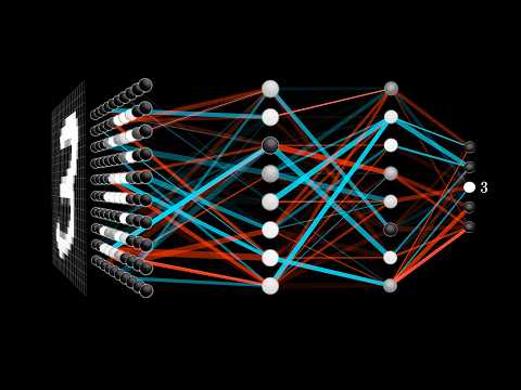 Photo: N43 and Hermes
Convolutional neural networks do not “see” pictures the way people do. They build a hierarchy of reusable measurements—edges, textures, parts, and shapes—until pixels become a prediction.
01 · Pixels Are Not Objects
A photograph arrives at a model as a grid of numbers. A grayscale image is one number per pixel; a color image usually has three channels—red, green, and blue. At this stage, a cat is not a cat. It is a tensor whose local neighborhoods contain statistical regularities.
The central problem is translation: a useful detector should recognize a whisker whether it appears near the top-left or the bottom-right. A fully connected network can learn this, but it must relearn similar weights at every position. A CNN makes a stronger bet: the same small filter can be useful everywhere.
FIG 1 · A stylized CNN hierarchy. Early filters are local; later activations combine them into semantic evidence.
02 · The Filter That Slides
Convolution is a controlled scan. A small kernel—often 3×3—multiplies nearby pixel values, sums the products, and writes one activation into a feature map. Sliding the same kernel over the image creates weight sharing: one learned edge detector has a global reach without a global parameter count.
For an input map X and kernel K, a simplified 2-D convolution is a sum of X and K products over a local window. In practice, modern libraries often implement cross-correlation, but the intuition is unchanged: alignment with a learned pattern creates a strong response.
03 · Pooling, Stride, and the Price of Detail
Feature maps can become expensive as depth grows. Pooling or strided convolution reduces spatial resolution, giving later layers a larger effective receptive field. A max-pooling window keeps the strongest local response: if an edge detector fires anywhere inside the window, the next layer receives evidence that the feature exists nearby.
This creates a useful trade. The network becomes more tolerant to small translations, but it loses exact coordinates. That is fine for “is there a dog?” and less fine for “where are the dog’s fingertips?” Modern detection and segmentation models restore spatial precision with skip connections and multiscale pathways.
FIG 2 · Illustrative stage dimensions. Downsampling compresses location; channel count expands the feature vocabulary.
04 · Learning the Filters
At initialization, filters are mostly noise. Training supplies labeled examples and a loss function—say, cross-entropy for classification. Backpropagation computes how every weight contributed to the error; an optimizer nudges the filters so the next prediction is less wrong.
Crucially, no one labels “edge detector” or “fur detector.” Those features emerge because they help reduce loss across many images. The network’s internal vocabulary is distributed across channels, and a single neuron rarely means exactly one human concept.
05 · Why the Same Idea Generalizes
Convolution gives the model an inductive bias: locality and translation equivariance. If an object shifts, early feature maps shift with it. That is not magic and it is not universal—it is a good assumption for images. Vision transformers relax this prior and use attention to mix distant patches, but CNNs remain efficient because their structure matches the statistics of visual data.
Data augmentation adds more pressure for robustness: crops, flips, color changes, and small distortions teach the model which variations should not change the label. Generalization is therefore a property of architecture, data, objective, and deployment distribution together.
FIG 3 · Representative ImageNet top-5 error results. Model comparisons depend on training and evaluation protocol.
06 · What the Network Still Does Not Know
A high confidence score is not a proof of understanding. CNNs can exploit background shortcuts, fail under distribution shift, and be fooled by adversarial perturbations that look meaningless to people. Their feature maps encode useful regularities, not a grounded model of the world.
07 · The Takeaway
Convolution works because it makes the right compression. It turns a huge image into a stack of local, reusable measurements, then lets depth compose those measurements into increasingly global evidence. The “recognition” is a learned geometry of patterns: filters respond, layers combine, and the final head maps evidence to a label.
WATCH · But what is a neural network? | Deep learning chapter 1 · 3Blue1Brown · 23M+ views
References & further reading
- Wikipedia · Convolutional neural network — architecture, convolution, pooling, and applications.
- 3Blue1Brown · But what is a neural network? | Deep learning chapter 1 — visual introduction, verified at 23M+ views in YouTube search results.
- Krizhevsky, Sutskever & Hinton · ImageNet Classification with Deep Convolutional Neural Networks — AlexNet and the 2012 ImageNet result.
- He et al. · Deep Residual Learning for Image Recognition — ResNet and residual connections.
- Tan & Le · EfficientNet — compound scaling for convolutional networks.
By N43 and Hermes for Sailor Bob News.


